Digital filters for live signal processing in Python

Digital filters are commonplace in biosignal processing. And the SciPy library offers a strong digital signal processing (DSP) ecosystem that is exceptionally well documented and easy to use with offline data. However, there is shockingly little material online on DSP in Python for real-time applications. In a live graphical interface (like yarppg), the signal needs to be processed while it is being generated - one sample at a time.

In this post, I am showing two different implementations of digital filters, that can be used in a real-time setting. DSP is a vast topic - the theory behind it involves many topics that I only understand superficially: trigonometry, linear time-invariant (LTI) systems, transformations to the frequency spectrum domain, etc… I will not try to explain these concepts but rather focus on the application in Python. A great resource to learn more about DSP is dsprelated.com.

This post covers the following topics:

• live implementation of digital IIR filters equivalent to SciPy’s lfilter
• adding live filters to the code from the earlier post on yarppg
• brief intro to second-order sections (SOS filters)
• live implementation of digital IIR filters equivalent to SciPy’s sosfilter

Live filter implementations in Python

I covered some of the basics on digital filters in my previous post, where I showed an example application of an infinite impulse response (IIR) filter from the SciPy library. Filter design and application is conveniently achieved in only two lines of code:

1
2
3
4

# Butterworth low-pass filter with frequency cutoff at 2.5 Hz
b, a = scipy.signal.iirfilter(4, Wn=2.5, fs=30, btype="low", ftype="butter")
# apply filter once
yfilt = scipy.signal.lfilter(b, a, yraw)

In a real-time setting, the incoming signal needs to be processed one sample at a time. So we want a representation of the filter where the following code is equivalent to the scipy filter functions:

1
2

# process values one sample at a time
yfilt = [livefilter(y) for y in yraw]

Base class for live filter implementations

As I am going to show two different implementations, I am defining a base class, that takes over some of the boilerplate. Arguably, it is not that much anyway, but this approach should improve extendibility:

 1
 2
 3
 4
 5
 6
 7
 8
 9
10
11
12
13
14
15
16
17

import numpy as np

class LiveFilter:
    """Base class for live filters.
    """
    def process(self, x):
        # do not process NaNs
        if np.isnan(x):
            return x

        return self._process(x)

    def __call__(self, x):
        return self.process(x)

    def _process(self, x):
        raise NotImplementedError("Derived class must implement _process")

By implementing the __call__ method, we can have the filter behave like a function while still being able to track the filter state as instance variables.

Difference equation implementation: lfilter-equivalent

A digital filter can be described using a difference equation. It looks like the following and defines the new output value $y[n]$ as a weighted sum of past inputs $x[n-k]$ and outputs $y[n-k]$: $$ a_0 y[n] = b_0 x[n] + b_1 x[n-1] + b_2 x[n-2] - a_1 y[n-1] - a_2 y[n-2] $$ Once we have obtained the coefficients $b_k$ and $a_k$ from a filter design function (like scipy.signal.iirfilter), we can use the above equation to implement the filter. The filter class (LiveLFilter) needs to keep track of the most recent inputs and outputs to calculate the new output. The constructor looks as follows:

 1
 2
 3
 4
 5
 6
 7
 8
 9
10
11
12
13
14

from collections import deque

class LiveLFilter(LiveFilter):
    def __init__(self, b, a):
        """Initialize live filter based on difference equation.

        Args:
            b (array-like): numerator coefficients obtained from scipy.
            a (array-like): denominator coefficients obtained from scipy.
        """
        self.b = b
        self.a = a
        self._xs = deque([0] * len(b), maxlen=len(b))
        self._ys = deque([0] * (len(a) - 1), maxlen=len(a)-1)

Since we only need to track a moving window of input and output values, it is convenient to use a double-ended queue. The Python standard library provides an implementation of this data structure (collections.deque). The queues holding past x and y values are restricted to only hold as many values as needed in the difference equation. Then, whenever a value is pushed to the full queue, the oldest value is dropped.

In order to allow any filter order, and thus any length of coefficient vectors, I am using numpy functions for multiplications and additions. The difference equation can be rewritten as the difference of two dot products, all that is left to do is to append x and y values to the correct side of the queue. Note that by appending values from the left, the coefficients $b_k$ and $a_k$ are properly aligned with the past inputs $x[n-k]$ and outputs $y[n-k]$. If we used the more common append method, we would need to reverse one of the vectors inside the dot products.

1
2
3
4
5
6
7
8
9

    def _process(self, x):
        """Filter incoming data with standard difference equations.
        """
        self._xs.appendleft(x)
        y = np.dot(self.b, self._xs) - np.dot(self.a[1:], self._ys)
        y = y / self.a[0]
        self._ys.appendleft(y)

        return y

Also note that filter coefficients are typically scaled so that $a_0=1$. Line 6 above could be omitted, but I want the function to allow any coefficients.

LiveLFilter vs. SciPy’s lfilter

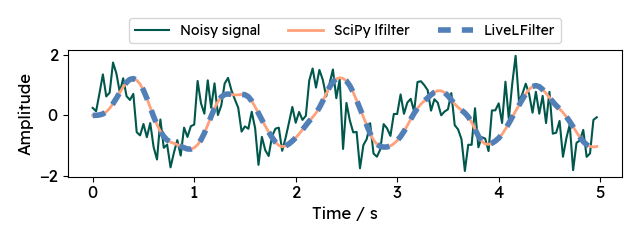
This was already the entire code for the LiveLFilter class. To see if the filter implementation works as expected, we can use the example signal from the last post. It is a 1 Hz sine wave overlaid with Gaussian noise.

 1
 2
 3
 4
 5
 6
 7
 8
 9
10

import numpy as np

np.random.seed(42)  # for reproducibility
# create time steps and corresponding sine wave with Gaussian noise
fs = 30  # sampling rate, Hz
ts = np.arange(0, 5, 1.0 / fs)  # time vector - 5 seconds

ys = np.sin(2*np.pi * 1.0 * ts)  # signal @ 1.0 Hz, without noise
yerr = 0.5 * np.random.normal(size=len(ts))  # Gaussian noise
yraw = ys + yerr

Now, we can define and apply the IIR filter using with both the live implementation and the SciPy version. I am using the mean absolute error (MAE) metric from scikit-learn to quantify the difference.

 1
 2
 3
 4
 5
 6
 7
 8
 9
10
11
12
13

import scipy.signal
from sklearn.metrics import mean_absolute_error as mae
from digitalfilter import LiveLFilter

# define lowpass filter with 2.5 Hz cutoff frequency
b, a = scipy.signal.iirfilter(4, Wn=2.5, fs=fs, btype="low", ftype="butter")
y_scipy_lfilter = scipy.signal.lfilter(b, a, yraw)

live_lfilter = LiveLFilter(b, a)
# simulate live filter - passing values one by one
y_live_lfilter = [live_lfilter(y) for y in yraw]

print(f"lfilter error: {mae(y_scipy_lfilter, y_live_lfilter):.5g}")

lfilter error: 1.8117e-15

The MAE is very close to zero and there is no visual difference between the outputs of both filters:

 1
 2
 3
 4
 5
 6
 7
 8
 9
10
11

plt.figure(figsize=[6.4, 2.4])
plt.plot(ts, yraw, label="Noisy signal")
plt.plot(ts, y_scipy_lfilter, lw=2, label="SciPy lfilter")
plt.plot(ts, y_live_lfilter, lw=4, ls="dashed", label="LiveLFilter")

plt.legend(loc="lower center", bbox_to_anchor=[0.5, 1], ncol=3,
           fontsize="smaller")
plt.xlabel("Time / s")
plt.ylabel("Amplitude")
plt.tight_layout()
plt.show()

Application of live filters in yarppg

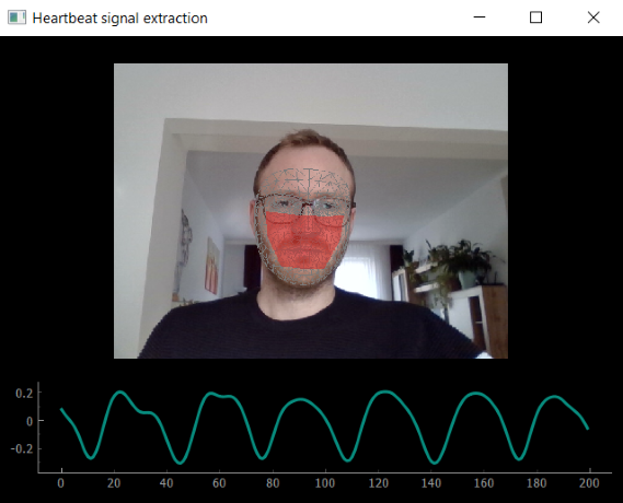
In my post on heartbeat signal extraction, I recreated a minimalistic version of yarppg, that obtained a rather noisy pulse signal from the webcam input. We can leverage the LiveLFilter implementation from above to process the raw pulse signal, reducing noise and removing lower-frequency drifts in the signal. The filter type to remove both lower and higher frequencies at the same time is called band-pass. It passes a specified frequency band while everything else is rejected.

Extension of previous code

First, let’s adjust the RPPG class to actually perform the filtering. I add a filter_function argument defaulting to None in the constructor. If nothing is passed here, a do-nothing lambda function is created:

1
2
3
4
5
6
7

class RPPG(QObject):
    def __init__(self, parent=None, video=0, filter_function=None):
        # ...
        if filter_function is None:
            self.filter_function = lambda x: x  # pass values unfiltered
        else:
            self.filter_function = filter_function

The provided filter function is then simply applied during on_frame_received. There is only one more line to adjust in RPPG:

1
2
3
4
5
6
7
8

    def on_frame_received(self, frame):
        """Process new frame - find face mesh and extract pulse signal.
        """
        rawimg = frame.copy()
        roimask, results = self.detector.process(frame)

        r, g, b, a = cv2.mean(rawimg, mask=roimask)
        self.signal.append(self.filter_function(g))

Now, all that is left is to define the band-pass filter and pass it to RPPG in the main function. For convenient creation of the live filter, a helper function is added to rppg.py:

 1
 2
 3
 4
 5
 6
 7
 8
 9
10
11
12
13

def get_heartbeat_filter(order=4, cutoff=[0.5, 2.5], btype="bandpass",
                         fs=30, output="ba"):
    """Create live filter with lfilter or sosfilt implmementation.
    """
    coeffs = scipy.signal.iirfilter(order, Wn=cutoff, fs=fs, btype=btype,
                                    ftype="butter", output=output)

    if output == "ba":
        return LiveLFilter(*coeffs)
    elif output == "sos":
        return LiveSosFilter(coeffs)

    raise NotImplementedError(f"Unknown output {output!r}")

The LiveSosFilter implementation, using second-order sections is discussed in a later section.

Final application

The new main function, initializing the components and starting the user interface, only needs two additional lines:

 1
 2
 3
 4
 5
 6
 7
 8
 9
10
11
12
13
14
15
16
17

# main.py
from PyQt5.QtWidgets import QApplication

from mainwindow import MainWindow
from rppg import RPPG, get_heartbeat_filter

if __name__ == "__main__":
    app = QApplication([])
    live_bandpass = get_heartbeat_filter(order=4, cutoff=[0.5, 2.5], fs=30,
                                         btype="bandpass", output="ba")
    rppg = RPPG(video=0, parent=app, filter_function=live_bandpass)
    win = MainWindow(rppg=rppg)
    win.show()

    rppg.start()
    app.exec_()
    rppg.stop()

Using the filter settings above, the extracted pulse signal is nicely smoothed and heart beats are more clearly visible. In the next post, we can tackle finding peaks in the pulse signal and computing an average heart rate.

Improving stability with second-order sections

According to the SciPy documentation, the function scipy.signal.sosfilt should be preferred over lfilter in pretty much all filtering tasks. This is because, in their normal form, IIR filters are susceptible to coefficient quantization errors and digital implementations can run into stability problems. ¹

Second-order sections filter (biquads)

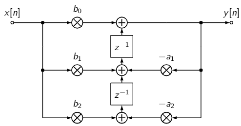
To combat the numerical problems of higher-order filters, an IIR filter can be broken down into a cascade of so-called second-order sections. Second-order sections (or biquads) can be designed in several different structures². The SciPy library works with the transposed direct form II shown below. The $z^{-1}$ blocks denote a one-sample delay.

The signal flow chart can be read like this: The biquad output $y[n]$ is calculated by adding $x[n]\cdot b_0$ and $w[n-1]$. Where $w[n-1]$ is the result of the summation in the center one sample ago (delayed in the $z^{-1}$ block). Any higher-order filter can be rewritten as a series of such biquads. As a user, we really do not need to care all that much about the mathematics behind this. A filter designed as cascaded biquads can be obtained with scipy.signal.iirfiler by setting the argument output="sos".

Live implementation of sosfilt

I am creating a second class derived from LiveFilter. In the constructor, we need to store the biquad coefficients and zero-initialize the state. Additionally, we get the number of filter sections from the coefficients' shape:

 1
 2
 3
 4
 5
 6
 7
 8
 9
10
11
12
13
14

class LiveSosFilter(LiveFilter):
    """Live implementation of digital filter with second-order sections.
    """
    def __init__(self, sos):
        """Initialize live second-order sections filter.

        Args:
            sos (array-like): second-order sections obtained from scipy
                filter design (with output="sos").
        """
        self.sos = sos

        self.n_sections = sos.shape[0]
        self.state = np.zeros((self.n_sections, 2))

It took me a while to get the code below working, after digging through the SciPy code and documentation as well as some other resources mentioned before (¹, ², ³ and ⁴). In essence, it’s actually less than six lines of code, but they are quite dense.

 1
 2
 3
 4
 5
 6
 7
 8
 9
10
11
12
13

    def _process(self, x):
        """Filter incoming data with cascaded second-order sections.
        """
        for s in range(self.n_sections):  # apply filter sections in sequence
            b0, b1, b2, a0, a1, a2 = self.sos[s, :]

            # compute difference equations of transposed direct form II
            y = b0*x + self.state[s, 0]
            self.state[s, 0] = b1*x - a1*y + self.state[s, 1]
            self.state[s, 1] = b2*x - a2*y
            x = y  # set biquad output as input of next filter section.

        return y

The for-loop iterates through all filter sections and computes the corresponding section output $y$. To make the code more readable and concise, the section coefficients are extracted into separate variables. Following the signal flow chart from above, the output $y$ is calculated as the sum of the current input $x$ (times $b_0$) plus the previous state of the first delay block. The first delay block in turn is given as the sum of three terms: $b_1 x$, $-a_1 y$ and the state of the second delay. Finally, the second delay block receives $b_2 x - a_2 y$. Note that delaying the signals occurs implicitly, as the previous values of self.state are accessed before they are computed for the current step. Before moving on to the computation of the next filter section, $x$ is overwritten by the biquad output. This imitates the next biquad being connected directly to the previous output.

LiveSosFilter vs. SciPy’s sosfilt

To make sure that the implementation works as intended, we can compare SciPy’s sosfilt output to the LiveSosFilter. Using the same example signal as above, we can simulate the live setting and compute the MAE.

 1
 2
 3
 4
 5
 6
 7
 8
 9
10
11
12
13
14

import scipy.signal
from sklearn.metrics import mean_absolute_error as mae
from digitalfilter import LiveSosFilter

# define lowpass filter with 2.5 Hz cutoff frequency
sos = scipy.signal.iirfilter(4, Wn=2.5, fs=fs, btype="low",
                             ftype="butter", output="sos")
y_scipy_sosfilt = scipy.signal.sosfilt(sos, yraw)

live_sosfilter = LiveSosFilter(sos)
# simulate live filter - passing values one by one
y_live_sosfilt = [live_sosfilter(y) for y in yraw]

print(f"sosfilter error: {mae(y_scipy_sosfilt, y_live_sosfilt):.5g}")

sosfilter error: 0

The output of the live implementation exactly matches SciPy’s implementation. In order to use LiveSosFilter instead of LiveLFilter in the live GUI, we only need to replace the output argument in get_heartbeat_filter to "sos". Although arguably in this specific application, there should not be a notable difference.

1
2
3

# in main.py
live_bandpass = get_heartbeat_filter(order=4, cutoff=[0.5, 2.5], fs=30,
                                     btype="bandpass", output="sos")

Here is a link to download the entire code for this article with DownGit.

(References)