Finding peaks in noisy signals (with Python and JavaScript)

In many signal processing applications, finding peaks is an important part of the pipeline. Peak detection can be a very challenging endeavor, even more so when there is a lot of noise. In this post, I am investigating different ways to find peaks in noisy signals. We explore SciPy’s incredibly useful find_peaks and find_peaks_cwt functions and develop a rudimentary peak finding approach from scratch in JavaScript. The JavaScript implementation is used to drive an interactive visualization describing parts of the find_peaks hyperparameters.

Peak detection in Python using SciPy

For finding peaks in a 1-dimensional array, the SciPy signal processing module offers the powerful scipy.signal.find_peaks function. Using the function is fairly straight-forward, the more difficult part is finding suitable arguments for your specific use case. There are several different options that influence which and how many peaks are detected. The SciPy documentation has some elaborate notes on these parameters.

Definition of peaks

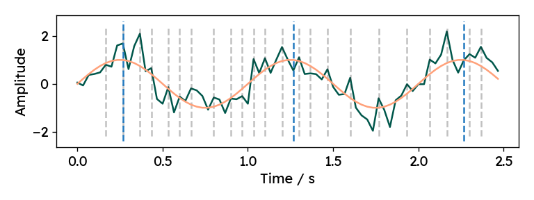
Before investigating the function arguments, we need to answer a more fundamental question: What is a peak? In the SciPy implementation, there is a single mandatory requirement for a sample to be labeled as a peak. A sample $y[k]$ is considered a peak, if the value is bigger than its two immediate neighbors (local maximum): $$ y[k] > y[k-1]\text{ and } y[k] > y[k+1] $$ Visually, it is evident, that this basic criterion may not be sufficient for noisy signals. Below is an example signal with all local maxima highlighted for a sine wave overlaid with Gaussian noise. Clearly, more constraints need to be imposed, in order to find only the relevant peaks.

Removing unwanted peaks with required properties

To filter the initial list of local maxima, we can define additional criteria. For example, in find_peaks we can specify the minimum distance between peaks, the minimum height and several more elaborate properties. Which criteria to use and what threshold values to choose heavily depend on the specific use case. Typically, you need to make some assumptions about the expected input signals in order to select useful parameters.

Let’s play around with two of these parameters to reduce the list of detected peaks. We are simulating seconds of a noisy signal pulsating with a frequency of Hz (recorded at 30 samples per second). Use the sliders below to investigate the effect of changing the corresponding values. Click “Refresh data” to generate a new random signal and test your settings on new data. Can you find a setting that works every time?

Depending on the frequency of the signal, different settings for the minimum distance can have wildly different effects. For a signal with frequency $f$, you would choose a minimum distance somewhere between $\tfrac{1}{2f}$ and $\tfrac{1}{f}$. But there should always be some breathing room for smaller deviations from the expected behavior. With minimum height, we can make sure that peaks below a certain threshold are not even considered as candidates. Values close to zero (50% of the peak-to-peak amplitude) are a good choice in the above example. For those curious about the JavaScript implementation behind this visualization, continue reading until the end of this post.

scipy.signal.find_peaks provides several more criteria for peak selection, which are fairly well described in the documentation. For example, peak width and peak prominence look not only at the single sample with the local maximum but also at the signal shape around the peak.

Peak detection in noisy signals

Some peaks in the example above are shifted off-center slightly. They do not properly align with the underlying signal frequency. This is a common issue when noise is present. If we are not interested in the exact location of the highest values but rather in the centers of the waves, we need to deal with the noise. The SciPy package provides the find_peaks_cwt function, which looks for peaks in several smoothed versions of the original signal¹. Here, CWT stands for continuous wavelet transform, which is a signal processing tool used in various applications from compression to biosignal analysis.

Alternatively, we can explicitly apply a lowpass filter and find peaks in the smoothed signal. I showed how digital filters can be applied in Python in my previous post. Let’s compare find_peaks_cwt and explicit smoothing with a synthetic signal. First, I am creating an example signal.

 1
 2
 3
 4
 5
 6
 7
 8
 9
10
11

import numpy as np

np.random.seed(256)  # for reproducibility

# create time steps and corresponding sine wave with Gaussian noise
fs = 30  # sampling rate, Hz
ts = np.arange(0, 8, 1.0 / fs)  # time vector - 8 seconds

ys = np.sin(2*np.pi * 1.0 * ts)  # signal @ 1.0 Hz, without noise
yerr = 0.5 * np.random.normal(size=len(ts))  # Gaussian noise
yraw = ys + yerr

Next, we define a bandpass filter, that removes the noise.

1
2
3

sos = scipy.signal.iirfilter(4, Wn=[0.1, 2.5], fs=fs, btype="bandpass",
                             ftype="butter", output="sos")
yfilt = scipy.signal.sosfilt(sos, yraw)

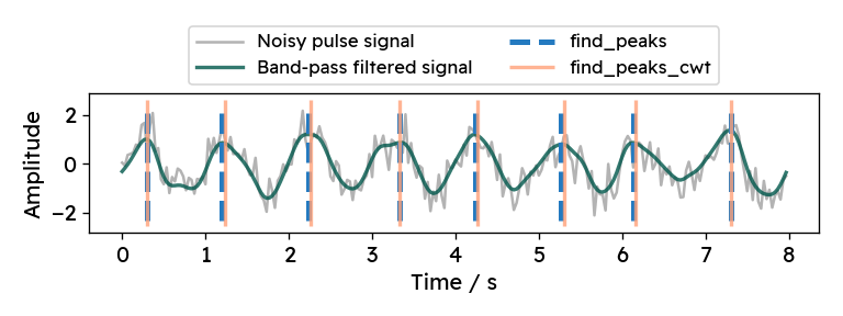
Now, we can apply both peak finding methods and visualize the results. For this example, I hand-picked the function parameters to work reasonably well with simulated pulse rates between 50 and 150 bpm (beats per minute). For the regular method (find_peaks) applied to the smoothed signal, the minimum allowed distance is set to 0.35 seconds, which corresponds to a maximum pulse frequency of roughly 170 bpm. By additionally setting the minimum peak height to 0, smaller random peaks (like the one at around 0.8 seconds in the image below) are neglected.

For the wavelet-based method (find_peaks_cwt), we can specify the widths parameter. The provided widths correspond to different levels of smoothing (wavelet width). According to the documentation, widths should include the expected peak width. For various signal frequencies, I found widths=np.arange(5, 15) to work well. A minimum width of 5 samples corresponds to 0.167 seconds, which is roughly half of the cycle time with a frequency of 170 bpm. At the other end, a width of 15 samples correspond to a peak width of 0.5 seconds. Choosing larger widths for this example signal leads to the algorithm missing some peaks.

1
2
3
4

# find peaks in smoothed signal
peaks, props = scipy.signal.find_peaks(yfilt, distance=0.35*fs, height=0.0)
# find peaks in noisy signal using wavelet decomposition
cwt_peaks = scipy.signal.find_peaks_cwt(yraw, widths=np.arange(5, 15))

Both methods work quite well and the corresponding outputs are almost identical.

Computational costs of find_peaks and find_peaks_cwt

When choosing between the two, one important factor to consider is computational effort. We can compare the two approaches using IPython’s %timeit magic. For the 8 seconds of signal from before, using find_peaks with explicit smoothing is roughly 4 times faster´ (even when including the filter design). For longer signals, the difference becomes even more severe. So if computation speed is an issue for your application, you might prefer the first option.

1
2
3
4
5
6
7

%%timeit
sos = scipy.signal.iirfilter(2, Wn=[0.1, 2.5], fs=fs, btype="bandpass",
                             ftype="butter", output="sos")
yfilt = scipy.signal.sosfiltfilt(sos, yraw)
peaks, props = scipy.signal.find_peaks(yfilt, distance=0.35*fs, height=0.0)

#> 749 µs ± 4.3 µs per loop (mean ± std. dev. of 7 runs, 1,000 loops each)

1
2
3
4

%%timeit
cwt_peaks = scipy.signal.find_peaks_cwt(yraw, widths=np.arange(5, 15))

#> 3.47 ms ± 17.4 µs per loop (mean ± std. dev. of 7 runs, 100 loops each)

Peak filter implementation in JavaScript

For the interactive chart above, I had to implement some parts of the find_peaks method in JavaScript. It’s impressive to see how much code is wrapped by a single line from the SciPy library — and I did not even implement all features of find_peaks.

Finding local maxima and filtering by height

The first step of the find_peaks approach is fairly straightforward: we need to find all local maxima. This is achieved by iterating through the input signal and taking note of all indices where the signal value is higher than both immediate neighbors.

 1
 2
 3
 4
 5
 6
 7
 8
 9
10
11
12
13
14

/**
 * Get indices of all local maxima in a sequence.
 * @param {number[]} xs - sequence of numbers
 * @returns {number[]} indices of local maxima
 */
function find_local_maxima(xs) {
    let maxima = [];
    // iterate through all points and compare direct neighbors
    for (let i = 1; i < xs.length-1; ++i) {
        if (xs[i] > xs[i-1] && xs[i] > xs[i+1])
            maxima.push(i);
    }
    return maxima;
}

Next, we can filter the local maxima by the minimum peak height and minimum peak distance. SciPy is explicit about the order of these operations. Computationally less intensive operations are performed first, so that more complex filters need to deal with fewer indices. Filtering by peak height can be done in one line in JavaScript, but it is cleaner to define a function anyway:

 1
 2
 3
 4
 5
 6
 7
 8
 9
10

/**
 * Remove peaks below minimum height.
 * @param {number[]} indices - indices of peaks in xs
 * @param {number[]} xs - original signal
 * @param {number} height - minimum peak height
 * @returns {number[]} filtered peak index list
 */
function filter_by_height(indices, xs, height) {
    return indices.filter(i => xs[i] > height);
}

Here, I am using the built-in Array.filter in combination with an arrow function. You can find more insights on filter and arrow functions here.

Filtering local maxima by minimum peak distance

Removing peaks that are too close to bigger ones is a bit more tricky and cannot be achieved in a single line. I had to dig through the SciPy code to get this right and adapted the code only slightly. The key idea of the code below is to go through the list of peaks from highest to smallest, identify all smaller peaks in the immediate surrounding of the current one (defined by the minimum distance) and mark them for removal.

For this to work, we need to be able to access the peak indices array from a second perspective: with decreasing height. In Python, I would use the numpy.argsort function, to get the order in which to access the peaks. Thankfully, I found a 3-line JavaScript implementation on StackOverflow:

1
2
3
4

// https://stackoverflow.com/a/65410414/10694594
let decor = (v, i) => [v, i]; // combine index and value as pair
let undecor = pair => pair[1];  // remove value from pair
const argsort = arr => arr.map(decor).sort().map(undecor);

Given a list of values, argsort returns an array with indices indicating how we would access the list in increasing order. Here is an example:

1
2

argsort([80, 40, 10, 60, 20])
/* returns [2, 4, 1, 3, 0] */

argsort tells us that we can find the smallest value (10) at position 2 of the input array (zero-indexed), the next bigger value (20) at index 4, etc.

Equipped with this tool, we can finally filter the list of peaks by minimum distance. Here is the full function, but I will break it down below.

 1
 2
 3
 4
 5
 6
 7
 8
 9
10
11
12
13
14
15
16
17
18
19
20
21
22
23
24
25
26
27
28
29
30
31
32
33

/**
 * Remove peaks that are too close to higher ones.
 * @param {number[]} indices - indices of peaks in xs
 * @param {number[]} xs - original signal
 * @param {number} dist - minimum distance between peaks
 * @returns {number[]} filtered peak index list
 */
function filter_by_distance(indices, xs, dist) {
    let to_remove = Array(indices.length).fill(false);
    let heights = indices.map(i => xs[i]);
    let sorted_index_positions = argsort(heights).reverse();

    // adapted from SciPy find_peaks
    for (let current of sorted_index_positions) {
        if (to_remove[current]) {
            continue;  // peak will already be removed, move on.
        }

        let neighbor = current-1;  // check on left side of peak
        while (neighbor >= 0 && (indices[current]-indices[neighbor]) < dist) {
            to_remove[neighbor] = true;
            --neighbor;
        }

        neighbor = current+1;  // check on right side of peak
        while (neighbor < indices.length
               && (indices[neighbor]-indices[current]) < dist) {
            to_remove[neighbor] = true;
            ++neighbor;
        }
    }
    return indices.filter((v, i) => !to_remove[i]);
}

Before iterating through the peaks, we need to define some auxiliary arrays. With to_remove we can take note of all the peaks that are too close to bigger ones and can therefore be removed. heights gives us the peak heights which we can use to get the access order for the array iteration (stored in sorted_index_positions). Note that the argsort output is reversed, so that we can go from highest to lowest.

 8
 9
10
11

function filter_by_distance(indices, xs, dist) {
    let to_remove = Array(indices.length).fill(false);
    let heights = indices.map(i => xs[i]);
    let sorted_index_positions = argsort(heights).reverse();

Now, we iterate through the list of peaks, starting at the highest one, which is referred to as current below. If the current peak was already marked for removal, it can be skipped.

14
15
16
17

    for (let current of sorted_index_positions) {
        if (to_remove[current]) {
            continue;  // peak will already be removed, move on.
        }

From the current peak, we first look towards the left, jumping from peak to peak and marking them for removal. We go to the left until the distance from the current peak is larger than the user-specified minimum peak distance dist or we reach the start of the signal.

19
20
21
22
23

        let neighbor = current-1;  // check on left side of current peak
        while (neighbor >= 0 && (indices[current]-indices[neighbor]) < dist) {
            to_remove[neighbor] = true;
            --neighbor;
        }

You may be wondering, why there is no comparison of peak heights between the current and neighboring peak. This is actually not necessary because we are already going through the list from highest to lowest. And we cannot revisit a higher peak while checking neighbors, since all peaks close to previously processed peaks were already marked for removal.

The right side of the peak is checked in the same way.

25
26
27
28
29
30

        neighbor = current+1;  // check on right side of current peak
        while (neighbor < indices.length
               && (indices[neighbor]-indices[current]) < dist) {
            to_remove[neighbor] = true;
            ++neighbor;
        }

Finally, the original list of peak indices can be filtered according to the notes taken in to_remove.

31
32

    return indices.filter((v, i) => !to_remove[i]);
}

Putting the pieces together

With functions for identifying local maxima and reducing the list by minimum distance and height, we can create a function that provides at least part of SciPy’s find_peaks functionality. This is what I used to drive the interactive visualization above.

 1
 2
 3
 4
 5
 6
 7
 8
 9
10
11
12
13
14
15
16
17
18
19
20
21
22
23
24
25
26
27
28
29
30

/**
 * Filter peaks by required properties.
 * @param {number[]}} indices - indices of peaks in xs
 * @param {number[]} xs - original signal
 * @param {number} distance - minimum distance between peaks
 * @param {number} height - minimum height of peaks
 * @returns {number[]} filtered peak indices
 */
function filter_maxima(indices, xs, distance, height) {
    let new_indices = indices;
    if (height != undefined) {
        new_indices = filter_by_height(indices, xs, height);
    }
    if (distance != undefined) {
        new_indices = filter_by_distance(new_indices, xs, distance);
    }
    return new_indices;
}

/**
 * Simplified version of SciPy's find_peaks function.
 * @param {number[]} xs - input signal
 * @param {number} distance - minimum distance between peaks
 * @param {number} height - minimum height of peaks
 * @returns {number[]} peak indices
 */
function minimal_find_peaks(xs, distance, height) {
    let indices = find_local_maxima(xs)
    return filter_maxima(indices, xs, distance, height);
}

Conclusion

Noise is an ever-present challenge in signal processing. If we want to find peaks in noisy signals, we have several options, which are available out of the box in the Python ecosystem. find_peaks finds all local maxima in the signal and reduces the list based on user-specified criteria.

We explored the effect of the minimum peak height and minimum peak distance criteria, which can lead to good results. To deal with the noise, it may be beneficial to first smooth the input before applying peak detection. As an alternative, SciPy provides a wavelet transform-based approach find_peaks_cwt that is specifically defined to find peaks in noisy signals. Regardless of the approach, it is always required to make assumptions about the expected signal shape, in order to set meaningful hyperparameters.

Finally, I showed how parts of the find_peaks function work and reimplemented those parts in JavaScript. It’s amazing how much functionality is provided in SciPy, which is also easy to use and very well documented. Kudos to the maintainers for making this available.

If you want to build on this post, you can download the Python and JavaScript code from my GitHub or from here.

(References)